The main graph area and the navigation pane are blank when you first enter IR mode. You won’t see any data in the graph area(s) until you record an Impulse Response measurement or display an IR measurement* saved as a .wav file from the Data Bar. You can import measurements stored in .wav or .aiff files into Smaart's IR data library using the Import > Trace Data File command in the File menu or the Import Trace command in the Data Bar menu.
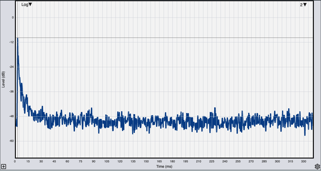
The larger (lower) portion of the IR mode graph area can be divided into one or two panes. Graph area allocation in IR mode works exactly the same way as the Real-Time mode graph area.
Each main graph pane can host any one of the six available main graph types:
Lin, Log, ETC (time Domain views)
Spectrograph (frequency and Magnitude vs time),
Frequency (Spectrum)
Histogram (bar chart of quantitative acoustics values by Octave or 1/3-Octave band.)
 The graph type for each pane is selected by means of the drop-list control in the upper left corner of the pane. The two arrowhead-shaped widgets that appear on the left of the edge of logarithmic time-domain graphs and on the spectrograph control the spectrograph Dynamic Range.
Some main graph types also have additional selector controls in their upper right corner that control display options specific to that graph
When one or more live measurements and/or stored data traces are present on a graph, the name of the frontmost trace in the z-axis stacking order (we also call this the top trace) appears in the upper right corner of the graph pane. If there are multiple data traces on the graph, you can cycle the z order of a graph forward or backward by pressing the [Z] key or [Shift] + [Z] or by using the Cycle Z Order Forward and Cycle Z Order Reverse commands in the Command menu. Clicking the down arrow widget next to the front trace name opens the Graph Legend.
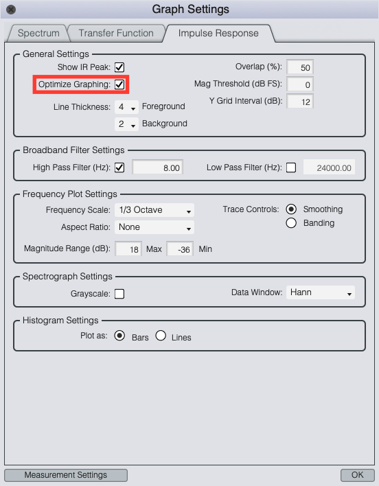
When multiple traces are displayed on time-domain graphs, they can be panned (moved horizontally) independently using the Time 0 widget in the navigation pane or by holding down the [Alt/Option] and [Shift] keys on your keyboard while pressing the [+/=] or [−] keys. Note that either action moves the front trace only. You can also align the highest peaks in all displayed traces to the highest peak in the front trace using the Sync Ld button in the Graph Legend or by holding down the [Shift] key on your keyboard while right-clicking on the graph with your mouse. Note that logarithmic time domain graphs (Log or ETC) may be easier to read when multiple IR measurements are displayed if you enable the Optimize Graphing option in Impulse Response Graph Settings, as shown in the screenshot above.
In addition to the graph type selector in the upper left corner of each pane, some of the graph types in IR mode have additional on-graph controls in the upper right corner:
The Frequency graph in IR mode has a menu in the upper right corner to select Smoothing (or optionally, Banding – see Impulse Response options) for the frequency response trace.
The IR mode Spectrograph display has on-graph controls for FFT size, Interval (FFT Overlap in milliseconds), Duration (how much of the time record to analyze, in ms) and fractional-octave Banding in the upper right corner, along with a Calc button that recalculates the spectrograph on demand.
The Histogram also has a menu in the upper right to select the data type and frequency resolution (Octave or 1/3 Octave) to display.
* Smaart can import .wav and .aiff files containing any type of audio data, but IR mode is purpose-built for analyzing impulse response measurements. There is no multi-channel file support or optimization for working with files more than a few seconds in length – and of course a lot of the IR analysis capabilities are irrelevant for other types of audio data.