The Spectrograph display in Impulse Response mode is essentially the same display as the real-time spectrograph only rotated 90° (with time on the x-axis instead of frequency). This is because the real-time mode spectrograph relates to other frequency-Domain graphs, but in IR mode we most often look at it alongside other time-domain graphs. The other main difference is that the number of “slices” in the IR mode spectrograph is determined by the currently selected FFT size and interval parameters.
To access the IR mode spectrograph, click the graph selector in the top-left corner of the plot and select Spectrograph. The spectrograph is initially calculated using the entire time range of the measurement or file being analyzed. If you don’t need to render the entire time record, you can click on the Duration value in the top-right corner of the graph and set it to a smaller value.
Changing the time range selection in the navigation pane does not affect the spectrograph as it does IR mode’s other time (Lin, Log, and ETC) and frequency domain graphs. However, panning or cropping the time record (or filtering the IR) will clear the spectrograph and require clicking the Calc button to plot the data again. You can resize the spectrograph and move its range using the [+], [−], and arrow keys. Alternatively, right-click-and-drag on the plot to zoom in to a selected range. Clicking in the margins of the plot will clear the zoom and return the plot to its default x/y range.
Time and Frequency Resolution
Each vertical stripe in the IR mode spectrograph represents one FFT, so in its simplest form (before applying frequency banding or time axis overlapping) the FFT size determines both the time and frequency resolution of the display. Larger FFTs provide greater detail on the frequency axis but may mask transient events on the time axis, so FFT size selection is a matter of weighting time against frequency resolution. The FFT and Interval controls that appear below the Calc button determine the time and frequency resolution of the spectrograph display.

FFT sizes ranging from 512 samples to 4K samples are compared at interval sizes approximately equal to the full FFT time constants (i.e., ≈ 0% Overlap). As the FFT size is increased, frequency resolution improves but the peak of the IR is smeared out over a wider time range. The x-axis of each graph is time (in ms), with frequency (in Hz) on the y axis.
The interval sizes selected for each FFT size represent the full FFT Time Constant rounded to the nearest millisecond, so there is essentially 0% overlap between “stripes.”

At 0% overlap, each FFT is calculated from unique data. At 50% overlap, the darker-shaded areas are shared by successive FFTs. Flattened half circles suggest a tapered FFT data window
The sharpest part of the peak in this impulse response (where most of the HF energy lives) is probably no more than a few milliseconds wide, but its energy is spread across the full FFT time constant in every case. At 512 points, time resolution (the FFT time constant) is a respectable 10.7 ms but FFT frequency bins are spaced 94 Hz apart. Increasing the FFT size to 4K points gets you 12 Hz frequency resolution but smears the peak in the IR out across an 85 ms time range.
Another parameter that can affect the spectrograph’s time resolution is the Interval setting. In the FFT size comparison (the 2×2 graphic), each successive FFT “slice” of the Spectrograph is calculated from nearly unique time domain data with each successive slice of time beginning approximately where the last one ended.
When the Interval setting is smaller than the full time constant of the selected FFT size, each successive FFT frame shares a percentage of its data with previous frames (see the above graphic). The FFT time constant is still the FFT time constant, but more overlap can sometimes restore some missing detail on the time axis as FFT size is increased, in addition to producing smoother blending between “slices” as you can see below.

The 2K FFT example from the previous section with approximately 50% (top), 75% (middle), and 90% (bottom) overlap.
The banding control in the bottom-right of the IR mode Spectrograph display applies fractional-octave banding to the frequency axis, reducing apparent frequency resolution, particularly in the high end. This can be useful in suppressing unnecessary detail to make larger features easier to see.
Dynamic Range

Spectrograph dynamic range and color mapping.
The Spectrograph’s dynamic range is controlled by two arrowhead-shaped widgets that appear on the top-left of the plot. These controls are echoed on the RTA graph when in Real Time mode or the Log IR and ETC displays when in IR mode. The level of each widget on these other plots correspond directly to their levels on the Spectrograph plot.
The top widget sets the maximum (Max) threshold; The lower one sets the minimum (Min). The Spectrograph scales its color spectrum between these two extremes. Any FFT bin whose Magnitude exceeds the specified maximum is mapped to the color white. Values falling below the minimum are mapped to black. These color mappings do not change when using a different skin. You can also specify threshold values for the Spectrograph’s dynamic range in the Spectrum tab of Graph Settings menu (Options > Graph Settings > Spectrum).
The key to creating a useful spectrograph is setting the dynamic range correctly. When the range is set too wide, the display loses definition and important features may become muddied. When set too narrow (or when the lower threshold is set too high) important features may be missed altogether. One of the major advantages of Smaart’s Spectrograph is its ability to adjust thresholds dynamically. This way, you can see the effects of different threshold values on data in real time and make comparisons.
Spectrograph Analysis of an Acoustical IR
Long-time Smaart users may recognize the impulse response measurement below as the room.wav file that was distributed with early versions of Smaart. The measurement was recorded on the stage of a 6000-seat performance space using an overhead PA cluster as the excitation source. It features a very prominent reverberant build-up Phase and problematic late reflected energy arriving about 160 ms after the direct sound.
This is a good file to see how changing the FFT size, Interval size, Banding and dynamic range can reveal different aspects of the IR measurement. In the example below, the navigation pane graph type is set to to ETC and has the Time set from 0 to about 100 ms. The FFT size is 2K, overlap is 95% and dynamic range is roughly -20 to -60 dB.
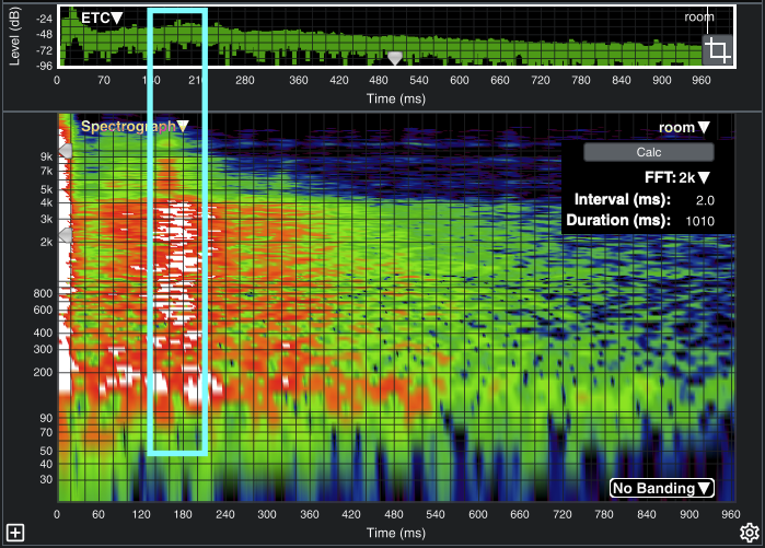
Broadband ETC and Spectrograph of a room impulse response showing a problematic back wall reflection. The spectrograph can be extremely useful for examining both the level and frequency content of features in the IR such as reverberant build-up and discrete reflections.