The main graph area can be divided into one or two graph panes (plus an optional Live IR pane for Transfer Function displays) by clicking the plus (+) button in the lower left corner of the graph when there is a single graph pane or a single main graph plus the live IR graph. When two or more graphs are displayed, an X button that appears in the same position (as shown below) that can be used to close an open graph pane. You can also use the main display buttons in the Control Bar View button menu to allocate the graph area, the way it was done in previous versions of Smaart.
When multiple graphs are displayed, one graph pane is always considered to be the active display. Clicking on a graph pane with your mouse selects it as the active graph pane and you can tell which pane is active by the color of the margins around the graph. In the figure below, the transfer function Magnitude graph in the upper pane is active, as denoted by its heavier, black border. When multiple windows are present, only one graph pane in the active window is active.
In Smaart RT, LE, and the Real Time mode in Smaart Suite, the active graph pane selection determines which set of live measurement controls you see in the Control Bar and which set of stored data you see in the Data Bar on the left the side of the window: Spectrum or Transfer Function. The active graph is also the source for data capture operations and keyboard or menu commands that affect what you see on a graph. Menu commands and keyboard shortcuts for zooming, moving traces, or cycling the z-order of multiple data traces all pertain to the active graph.

Main graph panes can be assigned any of the four real-time frequency chart types (RTA, Spectrograph, Transfer Function Magnitude or Phase) using the drop-down menu that appears in the upper left corner of each graph pane. For the Live IR pane you have your choice of three time Domain graph types: Impulse Response with linear or logarithmic Amplitude scaling or Envelope Time Curve (ETC).
Transfer function Phase and Magnitude graphs have logarithmic (fractional-octave) smoothing control in the lower left corner of each graph. Spectrograph and RTA graphs have a fractional-octave banding control in the same position. The (cog wheel) settings button in the lower right corner of each graph pane opens the Graph Settings page for the graph.
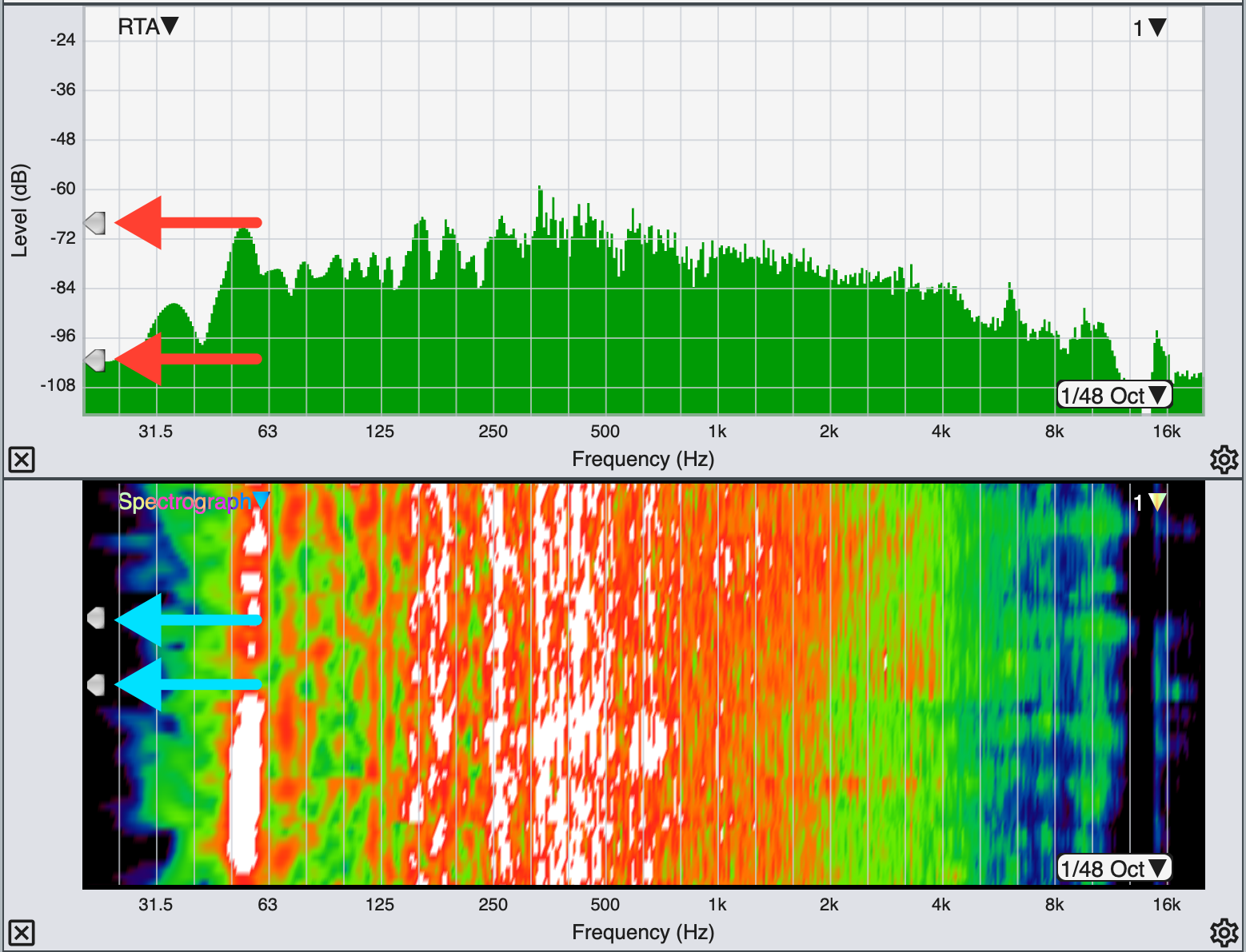
Real Time mode threshold slider widgets, indicated with arrows.
The arrowhead-shaped widgets that you can see positioned along the left edge of RTA and Spectrograph charts control the minimum and maximum threshold levels for the Spectrograph display. You can click on these and drag them up and down with your mouse to change the threshold levels. A similar widget positioned on the upper right edge of the transfer function Magnitude graph (see above) sets the coherence threshold for the coherence blanking feature, which removes data from the transfer function Phase and Magnitude graphs whose coherence values fall below the specified threshold level.
When one or more live measurements and/or stored data traces are present on a graph, the name of frontmost trace in the z-axis stacking order (we also call this the top trace) appears in the upper right corner of the graph pane. If there is a weighting curve applied to the measurement, the weighing curve name appears below the measurement name. You can also cycle the z order of a graph forward or backward by pressing the [Z] key or [Shift] + [Z] or by using the Cycle Z Order Forward and Cycle Z Order Reverse commands in the Command menu.
Clicking on the name of the front trace in the upper right corner of any real-time graph except the Live IR will open its legend box. The graph legend lists all live measurements that are currently displayed on the graph as well as any captured data traces (if applicable) that are currently visible. Please refer to the topic on Graph Legends for more details. Clicking anywhere in the Smaart window outside the legend box closes it.
Real Time Mode Plot Legends
Clicking on the name of the front trace in the upper right corner of any real-time graph except the Live IR will open its legend box. The graph legend lists all live measurements that are currently displayed on the graph as well as any captured data traces (if applicable) that are currently visible.

Live measurement traces appear in the legend as round buttons while captured traces are represented by file icons (a page with the corner folded over). One trace is always selected – normally the one at the top of the list – and the current active live measurement is indicated by an outline around it. Each icon in the legend is colored to match the display color of the corresponding data trace on the graph. If any trace has a weighting curve applied to it, a small bullet (•) is appended to the trace name to indicate this. When a trace is displayed with vertical (y-axis) offset, the offset value in decibels is shown to the right of the name. An inverted Transfer Function trace is shown with its name enclosed in curly brackets (e.g., “{Mic 1}”). Clicking anywhere in the Smaart window outside the legend box closes it.

Legend box for a transfer function graph
Clicking on the name of a live or captured trace in the legend box selects the object and moves it to the top of the legend list. This also makes it the top trace in the z-axis stack on the corresponding graph(s). You can multi-select traces in the legend box by holding down the [Ctrl/Cmd] key while clicking their names or by holding down the [Shift] key while clicking to select a contiguous group of objects.
You can hide a trace by clicking its icon in the legend. When you do this, the trace is removed from the graph and an “X” is drawn though its show/hide button on the Control Bar if it is a live measurement, or its icon in the data library pane on the Data Bar if it is a captured data file. Clicking on the icon or show/hide button for a hidden data file or live measurement removes the X and makes the trace visible on applicable graphs.
Below the legend list are three buttons. The Hide button hides a selected trace or group of traces and removes them from the graph. The Reset Y± button, clears all vertical offsets applied to any live or captured data trace. This action can be undone while the legend remains open by clicking the Reset Y± button again, provided that no additional changes have been made to trace offsets in the meantime. When two graphs of the same type are selected, the Move button moves the selected trace from the current graph to the other.
Plot Time Reference (PTR) and Time Offset (TO)
With Plot Time Reference enabled in Advanced Preferences, an additional control will appear in the bottom-left corner of any Phase plot(s) showing a number value (rounded to hundredths) and +/- buttons. The PTR value represents the Phase Plots Time Reference, or in other words, what that traces phase display is based on. The PTR is equal to the Measurement Time Reference of the captured trace, plus or minus any Time Offset applied using the PTR controls (using the +/- buttons). For example, the measurement below has a Measurement Time Reference (MTR) of 15ms, which the PTR text entry field reflects:

When you adjust the PTR value, that amount of delay is reflected as +/- Time Offset (TO) and displayed in the upper right corner of the Phase plot(s). The control and command concept here is meant to be similar to a Y-axis dB offset, the value of which is displayed in the upper-right of the Magnitude plot. The Phase Plot Legend will also display the TO value and has a button to clear TO. Below, the PTR value has been increased by .5ms. As now there is a Time Offset for that measurement, +0.50ms is displayed in the upper right corner of the phase graph. The PTR is now 15.50ms, however the MTR is still 15ms:

A key point here when describing what the phase PTR (Plot Time Reference) value is, is that it is the MTR +/- any Time Offset (TO): PTR = MTR +/- TO