Smaart’s GUI
The main window graphical user interfaces (GUIs) for Smaart software products all share a common basic design concept: data files on the left, main graphs in the center, controls on the right. At the top of the window are typical window control buttons (minimize, full-screen, restore to a floating window).
Windows software versions also have a menu bar within program windows – macOS versions follow the OS convention of putting the program's menu bar at the top of the screen – and both Mac and Windows versions have a tab bar that enables you to switch between multiple tabbed workspaces within a window with a single mouse click or screen tap. At the bottom of the window is a user-configurable button bar (the Command Bar) that you can customize to provide quick access to program functions that you use frequently.

The figure above denotes the common window areas and the names we use to refer to them. The contents of each area will differ according to the product type and if applicable, operating mode. Smaart RT, LE, and each have only a single operating mode to contend with. Smaart Suite has three – Real-Time, SPL, and Impulse Response.
The Tab Bar
Smaart can be run in multiple windows, each of which can in turn host multiple tabbed workspaces (or simply “tabs”). Each tab includes its own measurement assignments, screen layout, and data file show/hide selections. You can switch between them by clicking the tab-shaped buttons that appear below the menu bar:

To create, delete, rename, duplicate, or remove a tab, simply right-click the Tab Bar and select the appropriate option from the list:

You can also move a tab from one Smaart window to another by clicking on its button in the Tab Bar with your mouse and dragging it to another window, then releasing the mouse button to drop it.
If you are not using multiple tabs or are not switching between tabs very often, you can hide the Tab Bar to make a little more room for graphs either by selecting Tab Bar from the View menu or using the [A] hot key. Repeating either of these actions will restore the Tab Bar when it is hidden.
The Tab Bar command (keyboard shortcut: [A]) removes the tabs from the active Smaart window if they are currently visible or restores them if they were hidden. This can be a handy option for maximizing the space available for the graph area if you are not using multiple tabs.
Additional Options for Tabs/Windows
Smaart Suite contains a unique option for tabs under Advanced Preferences called “Operation Modes Open in New Window”. When enabled via checkbox, switching between Smaart’s different modes (or even between Spectrum and Transfer Function views) will create a new window in that mode or view. This can be helpful when switching back and forth between different types of data.

Smaart Suite and RT contain two additional options in this menu: "Stop Measurements on Tab Change” and “Stop Measurements on Mode Change”. These are both enabled by default and will cause any active measurement engines to stop running when changing tabs or switching between modes/views, respectively. Either or both of these can be disabled, if desired.
The Data Bar
The Data Bar provides easy access to captured measurement data. It can be shown or hidden by pressing the [B] key on your keyboard or selecting Data Bar from the View menu. When hidden, a triangular button appears in the left border of the window and clicking this button will restore it.

The Data Bar contains captured “snapshots” of real-time frequency-domain data traces known as “reference traces.” The type of data files shown on the Data Bar will depend on the current active graph selection. The Data Bar shows you only one type of data at a time, depending on the active graph selection in the graph area.
Smaart’s Real-Time Mode (Suite, RT, LE) shows one of two options depending on view:
When in Spectrum View, the Data Bar shows RTA traces in .srf format.
When in Transfer Function View, the Data Bar shows Transfer Function traces in .trf format.
Smaart’s SPL Mode (Suite, SPL) Data Bar shows SPL logs in .txt format.
Smaart’s IR Mode (Suite only) Data Bar shows Impulse Response measurements in .wav format.
The heading at the top of the Data Bar tells you which type of Smaart data files are currently shown. The (three-line) menu button in the upper right corner of the Data Bar a opens a menu of actions applicable to captured measurement data. This menu, along with the right-click (or [Ctrl]+click on Mac) context menu for the Data Bar, is covered in detail in the Data Bar Menus article. There is also a search bar that allows you to filter the data library based on your text entry. The filter is applied automatically as you type; to remove the sorting filter, simply delete the text entry or click the X icon to the right of the text.
The center portion of the Data Bar lists the files and folders in your current data library folder that match the active graph type. Each file icon is colored to match the display color for the data trace stored in the file. An “X” appears in the icons for files that are currently not being displayed on the active graph.
You can organize your data files using folders and drag files from one folder to another, much as you would in any file system window on your computer, and you can drag files from the data bar onto a compatible graph in the graph area to display them. Notice that one folder is always “pinned” to the top of the library pane. We refer to this folder as the “session folder.”
The session folder is the destination for new data captures and any new folders you create during your current Smaart session. You can change the session folder by clicking the (three-line) menu button in the upper right corner of the Data Bar and selecting New Session Folder from the menu, or by dragging an existing folder to the top position in the data library pane with your mouse and then releasing the mouse button. Creating a new session folder automatically changes the session folders for both {{glossary.Spectrum}} and transfer function data and the previous session folders become ordinary file folders. Dragging and dropping an existing folder to make it the session folder works similarly, except that the change applies only to the current data type.
At the bottom of the Data Bar are two buttons: Info and Delete. The Info button opens the Trace Info dialog for a selected data file, where you can review and edit file properties. You can also open Trace Info for a selected trace by pressing the [Enter] key on your keyboard. The [Esc] key can be used to close the dialog when it is open. Please refer to Trace Info Dialog for more details. The Delete button permanently deletes a selected file, folder, or group of objects selected in the library pane. You can select multiple files in the library pane, either by holding down the [Ctrl/Cmd] key while clicking on file icons with your mouse (to select an arbitrary group of files) or you can hold down the [Shift] key while selecting a contiguous range of objects. Note that deleting a folder automatically deletes all of the files and folders that it contains.
Working with Captured and Imported Data
Smaart has the ability to capture and display static “snapshots” of live spectrum, transfer function, and impulse response measurements as data files for later reference. Smaart v9 can open and display captured spectrum (.srf) and transfer function (.trf) data files from Smaart v7 and newer. You can also create Smaart RTA and transfer function data files by importing data in ASCII text format.
Captured and imported data traces are written to files in the designated session folder and will immediately appear in data library pane on the Data Bar. More information on Real Time Mode’s Data Bar’s menus cane be found here. Alternatively, information on Impulse Response Mode’s Data Bar can be found here.
Capturing Data from Live Measurements
You can capture new data trace files from live measurements on the active graph in the graph area by clicking the Capture or Capture All buttons. The Capture command (keyboard shortcut: [Spacebar]) captures the active live measurement on the active graph. Capture All ([Shift] + [Spacebar]) captures all currently running measurements that match the active graph type.
When capturing a single trace you will be prompted for a file name. Capture All prompts you for a folder name and then uses the names of the real-time measurements being captured as the filenames for the corresponding trace files.
Captured data files in the data library that are not currently displayed on a graph have an “X” drawn on their file icons. To display a hidden file or hide one that is visible, click its icon. Clicking on a data file’s name in the data library pane selects/highlights it. If the file is unhidden, this will also bring it to the top of the z axis on the active graph in the graph area. For details about a selected file, press the [Enter] key on your keyboard or click the Info button on the Data Bar to open the Trace Info dialog.
The Graph Area
The main graph area can be divided into one or two graph panes (plus an optional Live IR pane for Transfer Function displays) by clicking the plus (+) button in the lower left corner of the graph when there is a single graph pane or a single main graph plus the live IR graph. When two or more graphs are displayed, an X button that appears in the same position (as shown below) that can be used to close an open graph pane. You can also use the main display buttons in the Control Bar View button menu to allocate the graph area, the way it was done in previous versions of Smaart.
When multiple graphs are displayed, one graph pane is always considered to be the active display. Clicking on a graph pane with your mouse selects it as the active graph pane and you can tell which pane is active by the color of the margins around the graph. In the figure below, the transfer function Magnitude graph in the upper pane is active, as denoted by its heavier, black border. When multiple windows are present, only one graph pane in the active window is active.
In Smaart RT, LE, and the Real Time mode in Smaart Suite, the active graph pane selection determines which set of live measurement controls you see in the Control Bar and which set of stored data you see in the Data Bar on the left the side of the window: Spectrum or Transfer Function. The active graph is also the source for data capture operations and keyboard or menu commands that affect what you see on a graph. Menu commands and keyboard shortcuts for zooming, moving traces, or cycling the z-order of multiple data traces all pertain to the active graph.

Main graph panes can be assigned any of the four real-time frequency chart types (RTA, Spectrograph, Transfer Function Magnitude or Phase) using the drop-down menu that appears in the upper left corner of each graph pane. For the Live IR pane you have your choice of three time Domain graph types: Impulse Response with linear or logarithmic Amplitude scaling or Envelope Time Curve (ETC).
Transfer function Phase and Magnitude graphs have logarithmic (fractional-octave) smoothing control in the lower left corner of each graph. Spectrograph and RTA graphs have a fractional-octave banding control in the same position. The (cog wheel) settings button in the lower right corner of each graph pane opens the Graph Settings page for the graph.
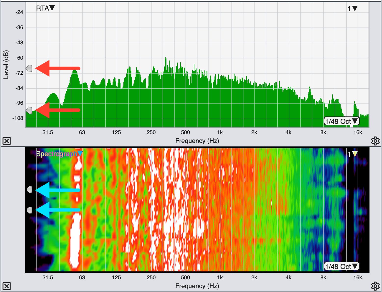
Real Time mode threshold slider widgets, indicated with arrows.
The arrowhead-shaped widgets that you can see positioned along the left edge of RTA and Spectrograph charts control the minimum and maximum threshold levels for the Spectrograph display. You can click on these and drag them up and down with your mouse to change the threshold levels. A similar widget positioned on the upper right edge of the transfer function Magnitude graph (see above) sets the coherence threshold for the coherence blanking feature, which removes data from the transfer function Phase and Magnitude graphs whose coherence values fall below the specified threshold level.
When one or more live measurements and/or stored data traces are present on a graph, the name of frontmost trace in the z-axis stacking order (we also call this the top trace) appears in the upper right corner of the graph pane. If there is a weighting curve applied to the measurement, the weighing curve name appears below the measurement name. You can also cycle the z order of a graph forward or backward by pressing the [Z] key or [Shift] + [Z] or by using the Cycle Z Order Forward and Cycle Z Order Reverse commands in the Command menu.
Clicking on the name of the front trace in the upper right corner of any real-time graph except the Live IR will open its legend box. The graph legend lists all live measurements that are currently displayed on the graph as well as any captured data traces (if applicable) that are currently visible. Please refer to the topic on Graph Legends for more details. Clicking anywhere in the Smaart window outside the legend box closes it.
The Control Bar
The Control Bar in real-time mode is home to live measurement controls for the active graph and signal generator. The Control Bar and in-tab SPL Meter (when present) can be shown or hidden by pressing the [O] key on your keyboard or selecting Control Bar from the View menu. When hidden, a triangular button appears in the right border of the window and clicking this button will restore it.
In Smaart Suite, three mode selector buttons appear above the control bar for switching between main display modes: Real-Time, Impulse Response, and SPL mode. You could say that Smaart RT and LE are always in real-time mode and Smaart SPL is always in SPL mode. In this topic, we will talk about the real-time control bar.

The in-tab SPL Meter/Clock can be hidden independently of the Control Bar, to make more room for live measurement controls. You can also change it to a clock by pressing the [K] key on your keyboard or selecting Toggle SPL/Clock from the View menu. To hide this display completely, use the SPL Meter command in the View menu or press [Alt/Option] + [K] on your keyboard.
Live Measurement Controls
The main section below the SPL Meter/Clock contains live measurement controls for the active graph (see Graph Area for more info). When the active graph is an RTA or Spectrograph, this area contains controls for Spectrum measurements. If the active graph is a Transfer Function, Magnitude, Phase Shift or Live IR graph, transfer function measurement controls appear here.

The label at the top of this section indicates which type of display (Spectrum or Transfer Function) is currently active. Notice that the label becomes a button when the mouse cursor hovers over it. Clicking this button opens the Measurement Settings dialog to the Spectrum or Transfer Function tab, depending on the current active display selection.

The Averaging control this section applies to the active live measurement, which is to say, the front-most live measurement on the active graph. The current active live measurement selection is indicated by the background color of its control block in the lower portion of the control strip. In the example shown here, measurement labeled “Mic 1” is active.
If the current active measurement uses the global settings for averaging, banding or smoothing (as applicable), changes to these settings will affect all measurements of the same type (unless otherwise specified). If the current active measurement is not subscribed to the global selections for a given setting, then the selector affects only the active measurement. A measurement engine’s parameters can be set independently from the global settings via the Spectrum Measurement Engine Settings fly-up menu. To access the fly-up, double-click the measurement engine you’d like to make changes to.
Below the active Averaging selector are tab-level measurement controls and individual control blocks for live measurement engines. Both spectrum and transfer function measurements have Stop All (■) and Run All (►) buttons that turn all measurements in the tab off or on as well as a Pause All button ( ▌▌). Note that the Stop All and Run All buttons are one-shot operations (clicking them a second time doesn't do anything) whereas the Pause All button latches; You click it once to pause and again to resume.
For transfer function measurements, the Track button turns delay tracking on for every measurement in the tab. The button to the right of it (with the stopwatch icon) triggers a timed measurement. The button labeled with the hammer and wrench icon opens the Measurement Config page.
The lower portion of the live measurement controls section is a scrollable area containing the control blocks for each individual measurement in the tab. If you have more measurement configured than can fit here, a scroll bar appears so that you can scroll through the list. The control blocks differ somewhat depending on the measurement type.
Live average control blocks (spectrum or transfer function) are the simplest. These consist of just the name of the measurement, a round Show/Hide button and a triangular Run/Stop button (►). The color of the Show/Hide button and the border color of the control block match the display color for the associated data trace on applicable graphs and their associated icons in Graph Legends. These elements are common to all types of live measurements.

To the above, we add an input level meter for single-channel spectrum measurements. Dual-channel transfer function measurements have two input level meters (labeled “M” and “R” for measurement and reference channel), a delay time field, and a delay-tracking indicator (●). You can click on the delay time field to make it editable and type in a new delay time (in milliseconds), then press the [Enter] key.
When a dual-channel transfer function measurement is the active measurement, an additional row of hover buttons appears below the base control set, labeled Find, Track, and −|+. The Find button starts the Delay Finder for the selected measurement, an automated routine for finding delay times for Signal alignment (see Activate Delay Finder for more on this). The Track button turns on delay tracking, which actively re-measures and adjusts measurement signal delay on each new update of the measurement – you can also turn delay tracking on and off by clicking the tracking indicator (●). The minus and plus (−|+) buttons decrease/increase the delay time for the measurement by one increment as specified in Transfer Function Measurement Settings. The default is one sample (about 21 microseconds per click at 48k Sampling Rate).
Clicking the Run button (►) for a live measurement starts the measurement, clicking it again when the measurement is running stops it. The run button turns green when the measurement is running and gray when it is stopped. Note that when you start a live average, at least one of the measurements that make up the averaged measurement must also be running in order to see any data on the graphs.
Notice that when you stop a live single-channel or dual-channel measurement, Smaart automatically hides it. If you unhide a stopped measurement, you will see the last data that it acquired on applicable graphs. This can be a handy way of “freezing” a trace for closer inspection without capturing a stored data trace.
The + Spectrum Engine and + TF Engine buttons below the live spectrum and transfer function measurement control blocks do the same thing as the New Spectrum and New TF commands in the Config menu. The View button opens a menu for selecting View Presets, which also includes main display control buttons for allocating the main graph area (à la Smaart 7 and 8, in case anyone misses them), Show/Hide buttons for the Data Bar, Tab Bar, Control Bar, and Command Bar, and a Tab selector drop list in case the tab bar is hidden. The Timer button opens the Timer Macro settings page.
The Command Bar

The Command Bar is a user-configurable button bar that runs across the bottom of a Smaart window. You can hide and restore it by means of the triangular button centered in the border area just above it. The show/hide button remains visible in the window border when the Command Bar is hidden and clicking this button again will restore it. You can also hide or restore the Command Bar by selecting “Command Bar” in the View menu or by pressing the [U] key on your keyboard. To customize the command bar, select “Command Bar Config” from the Config menu. Note that there are separate versions of the Command Bar; one for real-time spectrum and transfer function measurements and one for IR mode.
Configuring the Command Bar

Input The Command Bar consists of ten buttons, any of which can be assigned any one of a wide range of functions. In general, nearly anything you can do with a keyboard shortcut can also be done with a command bar button. Command Bar button functions are assigned in the Command Bar Configuration dialog, accessible by selecting “Command Bar Config” from the Config menu. There are two separate versions of the Command Bar; one for real-time spectrum and transfer function measurements and one for IR mode. Each has its own tab in the Command Bar Configuration dialog.
To assign a function to a Command Bar button, select the tab that you want to edit then click on one of the drop-list selectors in the Command column on the right and select the function that you want to assign from the list. A default name for the function will be automatically suggested in the corresponding Name field on the left. You can click on this field to make it editable if you want to change the name. After editing a button name, press the [Enter] key to set the change. When you are finished configuring your selections, click OK to exit the dialog. You should immediately see your new button name(s) on the corresponding Command Bar.