The Transfer Function Magnitude plot shows both the magnitude portion of the frequency response of the system under test (SUT) and coherence for the active transfer function measurement. The magnitude plot shows relative gain and Attenuation in the output of the system at each frequency.
If the reference and measurement signals are identical in level at all frequencies, the magnitude trace is a flat line at 0 dB. If there is an overall level difference between the two signals, the centerline of the measurement moves up or down on the graph – up means the measurement Signal is coming in at a higher level, relative to the reference signal, down means the reverse is true. If the SUT produces a relative gain at some frequencies and relative attenuation at others (as is usually the case with real world sound systems), the magnitude trace will deviate above the centerline of the measurement at frequencies where there is a relative gain and dip below it in regions of attenuation.
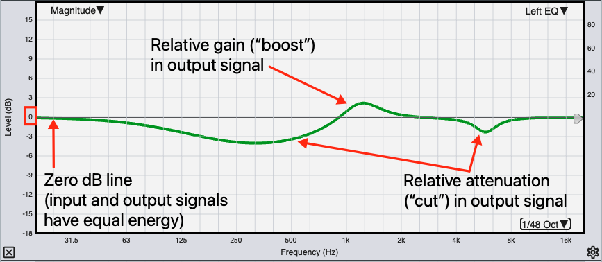
Transfer Function Magnitude plot.
Because we are directly comparing the signal going into the SUT to the output signal that the system produces in response, we get the same response curve using virtually any broadband signal with sufficient energy at all frequencies to resolve the measurement (including music). Unlike Spectrum measurements, the shape of the response curve is not dependent on the spectrum of the input signal. The resulting magnitude response ends up looking very similar to a fractional octave spectrum measurement made using Pink Noise, particularly when Polar averaging is used. When Complex magnitude averaging is selected, RTA and transfer function magnitude measurements of the same system can look significantly different in some cases, owing to the tendency for complex averaging to reject reverberation as “noise.“
When running multiple live transfer function measurements it is a good practice to match the sensitivity of each measurement so that that their overall magnitude levels match. This makes the overall levels of each measurement directly comparable to each other and directly relatable to relative sound pressure level. A straightforward method for sensitivity matching is to measure the same source from exactly the same position with each microphone, adjust their levels to match in that position and then don’t touch the preamp settings afterward. Of course, no two microphones have identical frequency response but any mic that bills itself as a measurement microphone should have very nearly flat response up to 10-12 kHz at least, so that is generally the range that you want to concentrate on most.
Note that sensitivity matching is not the same thing as sound level calibration. You could however, accomplish the more or less the same result using a sound level calibrator, by adjusting the input gains for each microphone to get the same full-scale for each. In that case, the calibration offset for SPL measurement would end up being the same for each microphone.
The Transfer Function Magnitude plot shows both the magnitude portion of the frequency response of the system under test (SUT) and coherence for the active transfer function measurement. The magnitude plot shows relative gain and Attenuation in the output of the system at each frequency.
If the reference and measurement signals are identical in level at all frequencies, the magnitude trace is a flat line at 0 dB. If there is an overall level difference between the two signals, the centerline of the measurement moves up or down on the graph – up means the measurement Signal is coming in at a higher level, relative to the reference signal, down means the reverse is true. If the SUT produces a relative gain at some frequencies and relative attenuation at others (as is usually the case with real world sound systems), the magnitude trace will deviate above the centerline of the measurement at frequencies where there is a relative gain and dip below it in regions of attenuation.
Transfer Function Magnitude plot.
Because we are directly comparing the signal going into the SUT to the output signal that the system produces in response, we get the same response curve using virtually any broadband signal with sufficient energy at all frequencies to resolve the measurement (including music). Unlike Spectrum measurements, the shape of the response curve is not dependent on the spectrum of the input signal. The resulting magnitude response ends up looking very similar to a fractional octave spectrum measurement made using Pink Noise, particularly when Polar averaging is used. When Complex magnitude averaging is selected, RTA and transfer function magnitude measurements of the same system can look significantly different in some cases, owing to the tendency for complex averaging to reject reverberation as “noise.“
When running multiple live transfer function measurements it is a good practice to match the sensitivity of each measurement so that that their overall magnitude levels match. This makes the overall levels of each measurement directly comparable to each other and directly relatable to relative sound pressure level. A straightforward method for sensitivity matching is to measure the same source from exactly the same position with each microphone, adjust their levels to match in that position and then don’t touch the preamp settings afterward. Of course, no two microphones have identical frequency response but any mic that bills itself as a measurement microphone should have very nearly flat response up to 10-12 kHz at least, so that is generally the range that you want to concentrate on most.
Note that sensitivity matching is not the same thing as sound level calibration. You could however, accomplish the more or less the same result using a sound level calibrator, by adjusting the input gains for each microphone to get the same full-scale for each. In that case, the calibration offset for SPL measurement would end up being the same for each microphone.