Delay Compensation
Delay compensation is a crucial factor in Transfer Function measurement. The reference Signal for the measurement, regardless of source, is typically a direct connection to our measurement system, meaning it travels through a piece of wire to the input of the measurement system at more or less the speed of light. The measurement signal (being the output of the system under test) is subject to delay from filtering, throughput delay in digital devices, intentional alignment delay, and of course in the case of acoustical measurements, Propagation Delay due to traveling through air at the Speed of Sound.
All of this can introduce tens of milliseconds of time offset between the reference and measurement signals and we must compensate for that offset by delaying the reference signal to match the arrival time of the measurement signal. Every two-channel transfer function measurement has a built-in delay line for just that purpose. Delay times for each live transfer function measurement are displayed directly to the right of a transfer function measurement engines input signal meters, and in the individual measurement settings . If you happen to know what the delay time should be for a given measurement you can enter it manually in either of these locations. Otherwise, we need to measure it.
Measuring Delays
There are multiple methods to find relative delay time between the two input signals (measurement and reference) in transfer function measurements. Most common are one of two automated routines (the Delay Tracker or the Delay Finder) which are based on locating peak energy arrival using Impulse Response measurements. In trickier cases, you can use the advanced delay finder. Experienced users also use the Phase display to fine tune delay times or deal with difficult cases such as subwoofer measurements in a noisy environment.
The Delay Finder
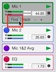
Delay Finder button.
Smaart’s Delay Finder is an automated routine for finding the relative delay time between the measurement and reference signals in the active transfer function measurement. It works by measuring the impulse response (IR) of the system under test (SUT) and then scanning the IR it to find the highest peak, which will normally represent the arrival of direct sound.
To measure delay, first ensure the the active graph is a Magnitude, Phase, or Live IR display so that the transfer function measurement controls are visible in the Control Bar. A quick way to accomplish this is by using the [T] hot key to enter the default Transfer Function view.
Next, click the measurement’s Run (play) button to start it. If the measurement is already running, clicking its control block in the Control Bar will select it as the active measurement. Ensure that the signal source being used to excite the SUT is turned on and input levels for the measurement are running at reasonable (and similar) levels.
The Delay Finder is accessible one of three ways:
The Activate Delay Finder command in the Command menu
The [L] hot key
Clicking the Find button on the control block for the active transfer function measurement on the Control Bar
After performing one of these three actions, the Delay Finder window will appear. Smaart will then calculate the delay time and display the result.
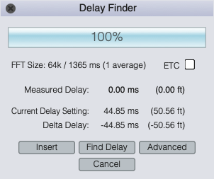
The Delay Finder dialog.
When the Delay Finder is run, Smaart automatically calculates the difference (Delta Delay) between the measured delay time and the current delay setting for the measurement. This is a handy tool for finding relative delay time between two loudspeaker systems (for example a main speaker and a delay speaker). For example:
Measure the furthest system away
Set the reference delay time to it
Mute that first system
Turn on the second system
Run the delay locator again, but do not insert the delay
Enter the resulting Delta Delay value in to second systems delay to align it to the furthest system away.
Selecting the ETC checkbox in the Delay Finder dialog tells Smaart to use the Envelope Time Curve (ETC) of the impulse response to find the delay time (rather than the linear peak of the IR). This will often result in a slightly different delay time but, depending on the scenario, one may provide a better answer than the other, especially when there is not significant high frequency information.
If the measured delay time seems reasonable and you are happy with the results, click the Insert button to assign the measured delay time to the current measurement and exit the Delay Finder dialog. If not, you can click the Find button to run the measurement again or click the Advanced button to access the Advanced Delay Finder and its functions (discussed below). Clicking Cancel exits the dialog without assigning the measured delay time.
The Delay Tracker
Smaart’s Delay Tracker feature is designed to keep transfer function measurements aligned in situations where the delay time may change from one measurement to the next. This can be the case, for instance, when measuring in windy conditions or when the microphone is being moved between captures/delay calculations such as when using Smaart's Timer Macro. It can also be used as a quick Delay Finder for measuring relatively short delay times under well-behaved measurement conditions. Just turn tracking on and let it find the delay time and lock on.
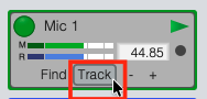
Delay Tracker button.
The Delay Tracker can be toggled on/off one of four ways:
The Toggle Delay Tracking command in the Command menu
Press the [D] hot key
Clicking the Track button on the control block for the active transfer function measurement on the Control Bar
Click on the circle/record button on a measurement engine control block
single click will engage the delay tracker, and then when the delay does not change for 3 consequtive measurement frames, it will automatically turn off
double-click will lock the delay tracker on, which is handy for moving the mic around or measuring in windy conditions.
The Delay Tracker uses a different FFT than the transfer function engine itself. Be default this is an 8k FFT, which has a time constant of 170ms (you can adjust this in Transfer Function Measurement Settings). At that size, the Tracker is very fast compared to the Delay Finder, whose default size is 64k (or 1365 ms). In practice, the Delay Tracker will always calculate delay times faster than the Delay Tracker as long as the expected delay time is about 60ms or less. With longer delay times, the Delay Finder will be a better choice.
The Delay Tracker is like a spotlight, as long as you are in the spotlight the tracker will see the direct arrival.
The Delay Finder, on the other hand, is more like a panoramic window and will see the direct arrival even if it is later in the time record.
You can increase the FFT size of both the Tracker (widen the spotlight) and the Finder in Transfer Function Measurement Settings.
The Advanced Delay Finder
Clicking the Advanced button in the Delay Finder dialog opens the Advanced Delay Finder window shown below. This window is resizable and “modeless,” so it can stay open while you work in other Smaart windows.

Advanced Delay Finder dialog.
The most obvious feature of the Advanced Delay Finder is its impulse response view of the active measurement instead of just the peak time. You can zoom in and out on this graph as you can any other graph in Smaart. The graph type selector in the upper-left corner gives you a choice of linear (Lin), logarithmic, (Log), or envelope time curve (ETC) plot type.
The cursor readout above the plot is formatted the same as Smaart’s other impulse response plots. In addition, it has fixed cursor coordinates on the left, movable cursor coordinates in the center, and the delta between the two on the right. You can move the fixed cursor position by holding down the [Ctrl/Cmd] key on your keyboard while clicking on the graph. When doing so, the found delay time will change to match the new position.
Clicking the Filter button in the upper-right corner of the graph runs a one-octave bandpass filter on the IR, centered on the frequency specified in the text entry field to the right of the button. This might be the crossover frequency between two systems that you want to align or any other frequency that you would like to isolate.
The control group in the lower left corner of the window presents the same information as the basic Delay Finder dialog. An IR measurement runs automatically when you open the Advanced Delay Finder, but you can re-run the measurement at any time by clicking the Find button. The Insert button inserts the found delay time as the reference signal delay for the selected transfer function measurement signal pair. Clicking the Store button adds the found delay time to the table to the right.
The table below the graph is a relative delay time calculator. Checking the T0 box next to any entry designates it as the time zero reference and recalculates all of the relative delta (Δ) time and distance figures for other entries accordingly. The up/down (▲|▼) buttons below the table move a selected entry up or down in its list. The Delete button deletes the selected entry and the Clear List button deletes all entries from the table.
The TF Pair selector to the right of the table enables you to select another transfer function signal pair to analyze. Note that changing this selection automatically re-runs the IR measurement. The level meters show you measurement and reference signal levels for the selected input signal pair. The Close button closes the window.
Delay Finder Measurement Parameters
The FFT size and number of averages for the Delay Finder are set from the Delay Finder section of Transfer Function Measurement Settings. The default is a 64K FFT with no averaging, which works out to a Time Constant of 1365 ms at a 48k sampling rate. This is sufficient for finding delay times at distances up to about 450 feet (140 meters) from a source.
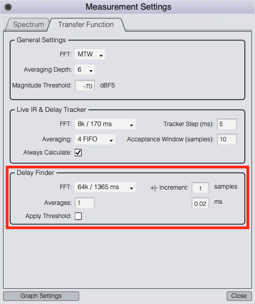
Delay Finder section of Transfer Function Measurement Settings.
As a rule of thumb, the FFT time constant should be least three times greater than the expected delay time. When measuring from extremely long distances or using a Sample Rate greater than 48k, you may need to increase the FFT size. When working in very noisy surroundings, increasing the number of averages may help as well.