A sound source’s positioning, orientation and directional characteristics will determine both its ability to cover an audience consistently and its propensity to excite non-audience areas of the room. The latter can enhance the listening experience if, for example, it adds a nice, clean “tail” of diffuse reverberation to an orchestral performance. But room excitation can also ruin the auditory experience if, for example; loudspeaker lobes are causing coloration or if loudspeaker arrays are poorly aimed causing late reflections, excessive reverberation and a loss of intelligibility.
Ignoring high frequency air absorption, a point source’s direct sound pressure will be inversely proportional to the distance between it and any given listening position (i.e. 1/r or 6dB Attenuation for every doubling of that distance). In echoic rooms, however, reverberation will add to the direct sound at the listening position depending on how directional the source is. An omnidirectional source positioned away from any boundaries would radiate sound pressure spherically and cause strong room excitation.
Directivity Factor (Q)
If a sound source is directional (such that its coverage is not fully spherical) its sound power gets concentrated into a smaller sector of a sphere. To help quantify that sound power concentration, sound sources are said to have a directivity factor (Q).
Directivity factor (Q) is:
1 for spherical source
2 for hemispherical source
4 for quarter spherical source…and so on.
Sound Pressure Level at the Listening Position
If we use directivity factor (Q) to quantify a sound source’s directional properties then, for on-axis listeners, the directivity-dependent relationship between source sound power level and the total (direct + reverberation) listener position sound pressure level approximates to:

The directivity factor (Q) can also be used to estimate the critical distance (Dc).

For the previous two equations:
Lp is the total (direct + reverberation) sound pressure level at the listening position
Lw is the source’s sound power level in dB referenced to 10−12 Watts
Q is the directivity factor (1 for spherical, 2 for hemispherical, 4 for quarter spherical etc.)
π is 3.142…
r is the distance between the source and the listening position
R is the room constant (the room’s ability to absorb sound – i.e. the product of surface area and absorption coefficient)
We don’t need to memorize these equations but understanding the relationship will help us troubleshoot problems. For instance, we see that:
Adding absorption will, obviously, reduce reverberation and increase the critical distance. Alternatively, we could reduce the effects of the reverberation by aiming highly directional loudspeakers into the audience (but away from the walls and ceiling).
Conversely, using fewer directional sources and/or lower room absorption (preferably with plenty of diffusion and a good balance between early and late decay times) will add “air” to our sound and prevent it from becoming too “dry.”
Directivity index (DI)
An alternative directivity figure that indicates the concentration of radiated power in dB is the Directivity Index (DI). Its value (in dB) is:

So, assuming the listener is on axis, if Q = 2, DI = +3dB; if Q = 4, DI = +6dB, and so on.
Q and DI figures in Practice
Large radiating surfaces tend to be more directional than small ones. Good far-field summation occurs perpendicular (on-axis) to large sources, and less-than-perfect summation occurs off-axis due to Phase variations between waves emanating from different areas of the surface. This can cause minor off-axis lobes at some frequencies and cancellations at others.
Courtesy: JBL Professional/Harman
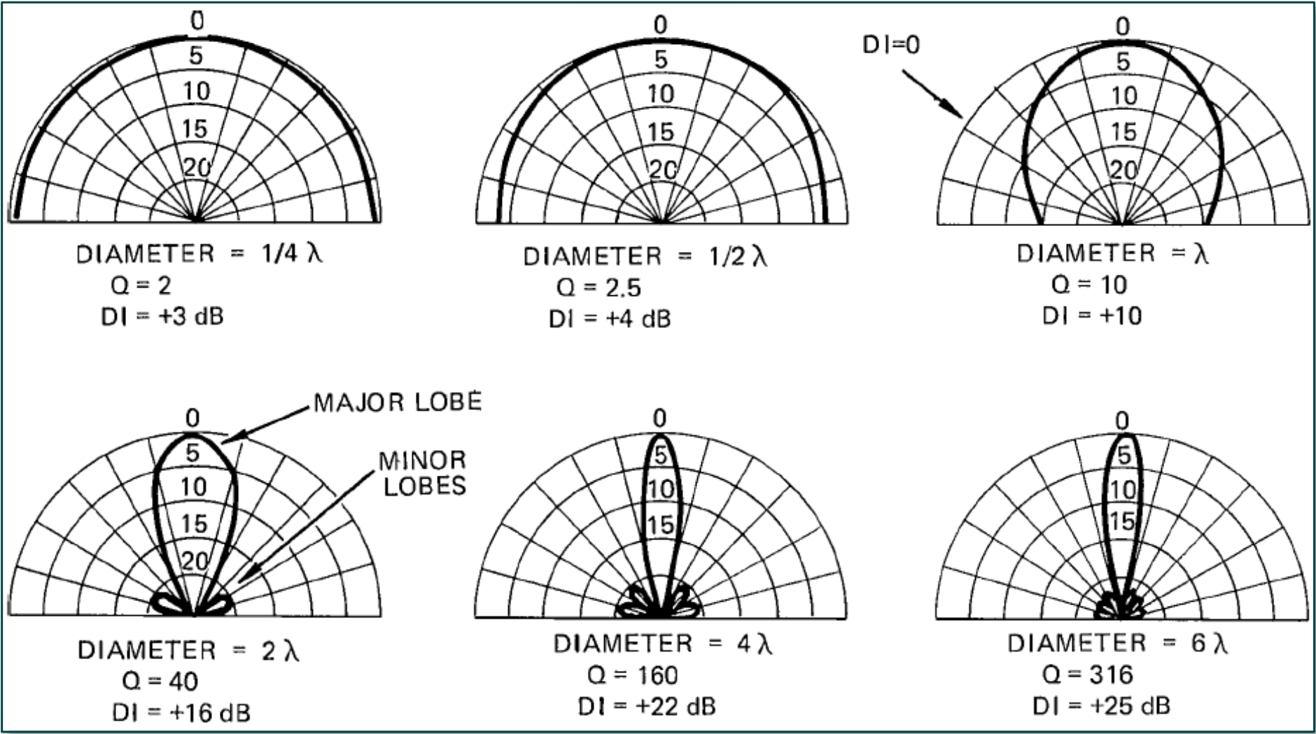
The above illustration shows the polar pattern, relevant directivity factor (Q), and directivity index (DI) of baffle-mounted piston-like sound sources (e.g. stiff loudspeaker cones) for various diameters, with respect to the wavelength of sound being produced.
Reading from left to right and top to bottom, you can either think in terms of an increasing diameter at a fixed frequency (or increasing frequency for a fixed diameter) for each successive example.
The nice thing about the directivity index figure DI is that it can be used in conjunction with a source’s polar plot (assuming a dB level scale) to indicate the true directivity index for an off-axis listener. This is shown in the top-right example above. The on-axis DI is +10dB, but, at the off-axis point (arrowed) the polar response is 10dB down with respect to the on-axis position. The DI at the off-axis point arrowed is the on-axis DI minus the off-axis figure – i.e., the off-axis DI is +10dB - 10dB = 0dB.
Conventional Loudspeaker Arrays
A spherical array of identical high-Q loudspeaker horns will act like one large spherical radiator if the optimum inter-cabinet splay angles are used. That being said, the array’s generally wider coverage will cause its overall directivity to be lower than that of the individual horns at mid and high frequencies.
At lower frequencies, however, arraying can provide tighter pattern control by making the system acoustically larger. Things can get quite complicated and pretty difficult to predict – especially when you factor in manufacturing tolerances, marketing-optimized loudspeaker specifications, inaccurate venue drawings, and a lively room’s sensitivity to relatively small changes in array shape and tilt.
Prediction software can get us close to our design goal and will certainly enable us to work out requirements, budgets, and other factors, but we need Smaart to check that installed systems are meeting spec. Smaart’s ability to complete as-built measurements – even during shows with an audience in place, if required – makes it a very powerful verification tool.
“Line” Arrays
It should be noted that the term “line” array has expanded in popular usage in recent years to become a term for a relatively long, vertical array of loudspeaker – typically just one cabinet wide. Manufacturers often imply that a line array system will give the user a textbook line-source radiation characteristic and many users assume they’ll benefit from a radial attenuation of 3dB/doubling of distance rather than the 6dB/doubling of a conventional array.
In reality, there is rarely the budget for a straight-line source column as it would have to stretch from the floor to the highest seat. Most “line” arrays are much shorter for budget and safety reasons and have to be progressively curved from top to bottom in order to cover the seating areas from the furthest, highest seat down to the front floor areas beyond the front fill coverage.
Luckily, the array’s upper, straighter part’s vertical pattern control can be very tightly controlled at mid and high frequencies. Additionally, if aimed hard into the audience, it can reduce upper wall and ceiling excitation, reducing the reverberant level and increasing the critical distance.
A Note about Echoes
The upper part of a line array provides tight mid-high pattern control above the array, minimizing direct ceiling excitation. However, the low radial attenuation rate can make them prone to creating very audible echoes from distant boundaries if they aren’t aimed accurately.
Always use Smaart’s linear (Lin) IR graph to check for echoes, as they can often be hidden amongst the room’s diffuse reverberation only to become audible, especially on stage, when the audience is in place and reverberant energy levels have dropped.
The line array effect of reducing radial attenuation from 6dB/doubling of distance to, say, 3 or 4dB/doubling of distance at mid-high frequencies can be illustrated as such:
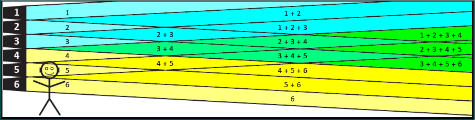
Imagine a listener is very close to just one horn-loaded element of the array. In the figure above, the listener (let’s call him Victor) mainly hears element 5, but with some minor off-axis contributions from the other elements.
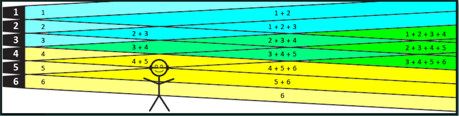
Each element (#1-6) is a point source and would, if measured in isolation, have the usual 6dB/doubling of distance radial attenuation characteristic. However, as Victor moves further away from element 5, he starts to benefit from the vector sum of elements 4 and 5 so the usual “6 dB/doubling” characteristic is modified by the extra element coming into play. This phenomenon is similar to the near field effect, mentioned earlier, which occurs close to any large sound source.
As Victor continues his journey further away from the array, he then benefits from the vector sum of more and more elements and these partially compensate for the usual 6 dB/doubling of distance that each element would have in isolation. Victor will benefit from this low (3-4 dB/doubling of distance) attenuation region any time there are extra elements available.
However, Victor will eventually run out of these extra elements, and the radial attenuation characteristic will revert back to the usual 6dB/doubling of distance. This point in Victor’s journey is called the transition distance, as shown in the next illustration.

Note that the transition distance, for a true line source, is proportional to frequency and to the line length squared.

Allowing for the fact that the Speed of Sound is temperature-dependent, transition distances for a typical 20 ft (~6m) straight long line source at 68° F (20° C) will be approximately:
Frequency | 200 Hz | 400 Hz | 800 Hz | 1600 Hz | 3600 Hz | 7200 Hz |
|---|---|---|---|---|---|---|
Transition Distance (ft) | 35.5 | 71.0 | 142 | 284 | 638.6 | 1277 |
Transition Distance (m) | 10.8 | 21.5 | 43.3 | 86.5 | 194.7 | 389.3 |
This suggests that high frequency propagation would be very efficient. But, in practice, HF energy will be significantly reduced by air absorption (by up to 0.1dB/meter, worse case) and, of course, imperfect coupling at high frequencies due to rigging tolerances.
It is particularly important to remember that transition distance is proportional to the square of the line length if spectral balance is to be maintained over a wide area. The length of the straight line section (at the top of most arrays) needs to be at least 6% of the maximum distance to be covered for spectrally balanced vocals.
The theoretical mid-high coverage pattern for a straight-line array narrows to a point (as shown in the table above) at the mid-array transition distance (although this varies with frequency), hence our need to curve real-world arrays for practical audience coverage. This is especially true where some audience members (like Victor) are below the maximum mid-array summation point: Victor’s ear-height transition distance is well beyond the mid-array transition distance in this case.
In practice, any temperature and wind gradients will move these transition points around significantly.
Beyond the transition distance there aren’t any elements available to compensate for any increase in listener distance, so the line array effect ceases to operate and the coverage “de-focuses” towards point-source-like behavior (with its 6dB/doubling radial attenuation characteristic).
Q: What has all this got to do with measuring room acoustics using Smaart’s Impulse mode?
A: Smaart’s ability to measure room phenomena “live” with an audience in place means that you will often be asked to assess acoustics under practical, amplified show conditions using an installed PA system. Many of these installed systems will be “line” arrays – whether appropriate or not – and a basic understanding of their properties will allow you to make intelligent recommendations.