Fractional octave smoothing of Transfer Function data is useful for to help make larger, more audible features and trends in data traces easier to see. Smaart offers two different smoothing functions for transfer function data: fractional octave and Frequency-Domain “Time Windowing” aka linear complex smoothing (what we simply call, “FTW”).
In general, fractional octave smoothing is the most useful and most commonly used of the two. However, there are specific applications where FTW can really come in handy, where a combination of the two provide the best results. More on that below, first let’s define the two.
Fractional Octave Smoothing
Fractional octave smoothing of transfer function data is analogous to fractional octave banding in an RTA measurement. In fact, if you pulled out just the frequencies from a log smoothed trace that correspond to fractional octave band centers and compared them to banded data, you would expect them to be almost identical. The main difference is that in the smoothed data trace, the “bands” overlap, preserving more detail than a bar graph or line trace.

Fractional-octave smoothing for transfer function data.
In a logarithmically smoothed data trace, each frequency data point is averaged with a varying number of frequency points on either side, depending on band size, frequency, and the frequency resolution of the underlying data. Because the data being smoothed is typically linearly spaced in frequency, the smoothing window widens logarithmically to include more and more adjacent points as frequency increases and the nominal band size grows larger. This helps to tame the HF “fuzziness” inherent in plotting FFT-based measurements of noisy signals on a logarithmic frequency scale, where excessive resolution (relative to how we humans hear) at higher frequencies combined with noise and other environmental factors can make the system response curve difficult to see.
Fractional octave smoothing of Magnitude data in Smaart runs directly on magnitude response data, as opposed to complex smoothing, where smoothing is performed on the complex transfer function data before magnitude is calculated. This tends to present the magnitude response in a way that correlates better with how we hear than complex-smoothed magnitude, which can suppress reverberant energy that may be audible and emphasize nulls in comb filters that may not be. Phase smoothing in Smaart is always based on complex data, to prevent “wrap” points from being averaged together.
FTW: Frequency-Domain Time-Windowing (aka Linear Complex Smoothing)
FTW smoothing is a linear (fixed bandwidth) smoothing function applied to the complex transfer function before magnitude and phase data are calculated. In this case, the bandwidth of the smoothing kernel is constant, rather than logarithmically expanding as frequency increases, which means the effects are most noticeable at lower frequencies.
Because the complex data includes both the time (phase) and magnitude response of the system, FTW smoothing affects both the magnitude and phase traces – there are no separate controls for magnitude and phase smoothing as there are for fractional octave smoothing. It is functionally equivalent to applying a data window function to the system Impulse Response (IR) in the time domain, limiting the effective Time Constant of the measurement, and then transforming the result back into the frequency domain using a zero-padded FFT.
Impulse response time windows are commonly used in acoustical analysis for such things as excluding problematic reflections from a measurement and/or isolating direct sound from a particular source –e.g., a loudspeaker under test – from later arriving energy emanating from other sources. When a time-windowed IR is transformed into the frequency domain, the practical result is a linear smoothing function, where some later-arriving noise along with comb filters resulting from any reflections that were windowed out are eliminated. FTW smoothing in Smaart emulates the frequency-domain resultant of windowing the IR in the time domain without requiring transforms back and forth between domains.

FTW Setting in the Control Bar once enabled in Advanced Preferences.
FTW smoothing in Smaart is applied only to transfer function data measured or captured with Complex magnitude averaging. It is considered an advanced feature that must be enabled in Options > Preferences > Advanced. Because all Smaart v9 transfer function engines calculate MTW, 32K (by default), as well as Polar and Complex Mag. Avg simultaneously - any data captured in the v9 platform may be viewed with FTW enabled (however, FTW is not a feature in Smaart LE).
FTW smoothing is specified in terms of the equivalent nominal half-window length in the time domain. When FTW is enabled, a text field for specifying the nominal window size (in milliseconds) and a checkbox to turn FTW on and off appear below the averaging depth controls for transfer function data on the Control Bar in the main Smaart program window(s). Because the equivalent window function in the time domain is fully symmetrical, the maximum half-window size is one half of the FFT time constant. As a general rule however, 25-30% of the FFT time constant might be considered a better practical maximum – e.g., 40-50 ms for an 8K FFT at 48000 samples/sec or 80-100 ms for 16K and so on.
Note that since FTW smoothing limits the effective Time Window of the transfer function measurement, the effective frequency resolution of the FTW-smoothed measurement depends on the nominal time window, not the time constant of the underlying FFT. For example, a 20 ms FTW window size always has an effective frequency resolution of 100 Hz, regardless of the FFT bin spacing, and data at frequencies below that point should be considered suspect or better yet, ignored. When FTW is turned on, a vertical red line appears on transfer function magnitude and phase graphs indicating this threshold frequency, based on the current nominal time window setting. More information on the relationship between time and frequency resolution can be found in Time and Frequency Resolution.
Using FTW and Fractional Octave Smoothing Together
A primary goal when working with Smaart data (or any data created by an audio analyzer), is to make that data best represenet what it is that you are actually trying to measure. In many cases, the impacts caused by a reflections of various frequencies at a measurement location can make the data traces we create difficult to parse - especially indoors, and especially in the lower frequencies where late-arriving reflections can cause our phase and magnitude traces to be quite challenged.
A solution to this, is to use linear complex smoothing (FTW) to clean up the low frequency, in combination with fractional octave smoothing to view a better frequency response trend that evens out middle and higher frequencies.
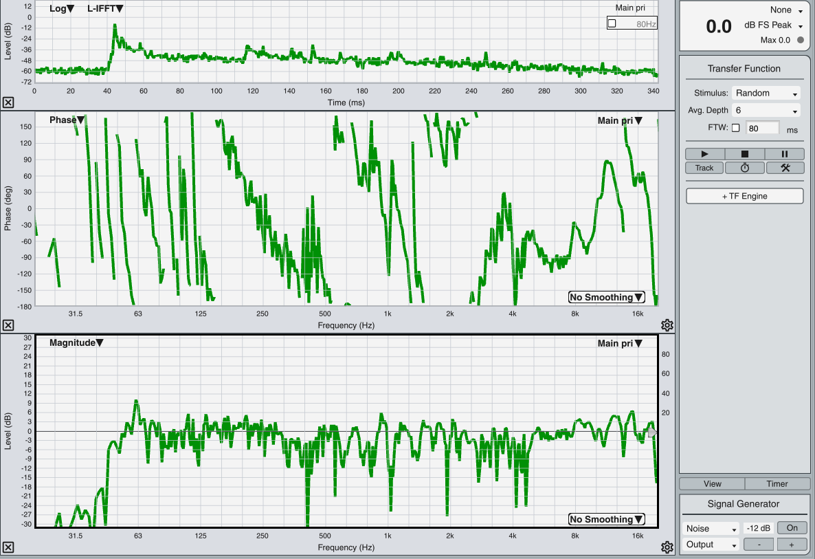
Below is a measurement in a challenging 1000 capacity seated indoor space with highly reflective solid brick walls throughout. This measurement has no fractional octave or FTW smoothing applied - notice the reflections in the L-IFFT view (enable L-IFFT view in Advanced TF Preferences) at 60ms, 120ms, 140ms, 150ms, etc. All of those reflections are cause the phase graph to show multiple breaks, and excessive ripple in the magnitude graph:
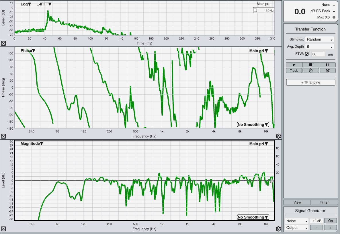
The following display is that same measurement, with 80ms of FTW applied. Notice that the LF has cleaned up significantly, and that in the Live IR plot the L-IFFT view shows that we’ve suppressed, or windowed out, a significant amount of energy - the trace goes off the screen by 160ms (80ms x2 =160ms!) .
Finally, here is the same measurement with both FTW and 1/6 oct smoothing applied. Using both techniques together maintains LF resolution while providing an HF response that is both easier to read, and representative of the tonality of the system. Using both techniques in tandem takes a fairly challenging single-point measurement, and turns it in to one that is much more approachable and easier to read.
